In this brief article, I introduce an ELO rating model and use it along with match data webscraped from thousands of matches, along with other predictive features to build a model using gradient boosting to predict the outcome (and implied probabilities) of historical cricket matches with a better results (lower logloss) than the Betfair exchange[1]

A trading strategy is implemented and backtested at the end of this introduction against 3 years of real match pricing with definitively market beating results.

I am currently live trading a similar but more complex system with trival amounts of capital for fun.

Repository Overview (Code):

Scraping and parsing for matches (including ball-by-ball match details), individual player rankings and player name mappings are performed in scripts located in cricstat.etl. These are saved to a local MySQL database.

Prior to re-training, new data must be synchronised from various online sources and linked by MatchId in the database. This is performed by running run_daily_process.sh, which calls various webscrapers..

Ingestion and linking Market pricing from betfair to above matches in databse from historical data is performed in marketdata.parse_betfair_historical.py

ELO model is build from match data in cricstat.train_elo_model and ML model trained in cricstat.train_model. A simple command line interface for live trading is at cricstat.livetrading.cli_trade_interface . This repository does not contain any fully automated trading code.

Explanation:

Before We Start Though – How Good is the Market at Predicting a Match Result?

Taking every international ODI match for which pricing is available (~4 years for Mens ODI cricket) and calculating the log loss of the implied probabilities versus actual winner yields 0.63. If we can built a predictive model which has a lower log loss than this, then in theory we are in general better than the market and can make profits in the long run by backing undervalued teams and laying overvalued teams. In reality there are additional factors which need to be taken into account such as transaction costs (the exchanges commision) and the liquidity of the market.

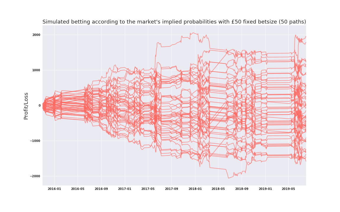
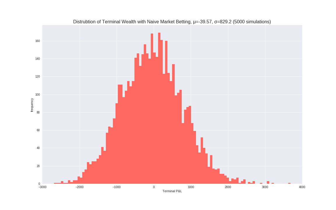
For the purposes of this simulation we use the final pre-match pricing available (usually a second or so before the match begins) First, lets see what would happen if we just bet according to market odds[2] to get an indication of how tight this market is using a fixed bet size each time:

Alternatively, consider a purely random bettor, who chooses which team to bet on based on a 50/50 coinflip.

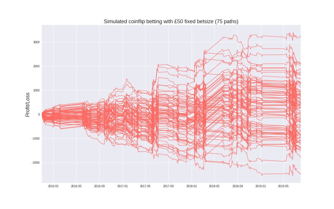
Pretty good, even with Betfair’s 5% commision on winning bets, this market is quite efficient, with the mean P&L of these simulations being very close to zero. As expected, playing this market in this way is not exactly a good idea for profitibility, however it is a much tighter market than I would have expected. P&L is roughly symmetrical around 0. The distribution of terminal income is roughly Gaussian as one would since these are effectively summations of many bernoulli trials.

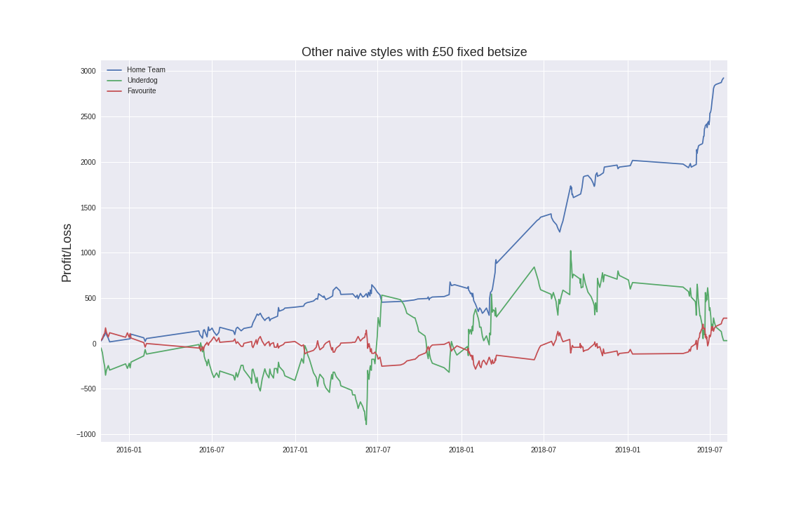
I ran various other naive simulations, such as always betting on the underdog/favourite

Note: Always betting on the home team appears to do very well around Summer 2019, this is due to the Mens ODI world cup where England won at home. Due to the relatively small sample size, the deceptively good P&L of this strategy should be viewed with caution.

I: ELO model:

Historical ICC team rankings are not easy to find and actually have less forward looking predictive power than i would expect on match outcome. As an alternative I built a rating system similar to that used by the World Chess Federation, the ELO system. Using all available match data for each format of the game (and by default starting each country’s ELO at 1500), we can iterate over (timestamp, Match) pairs and update the winning and losing teams ELO accordingly.

For an interesting read about the mathematics behind the rating system see this blog post.

ELO has a few hyperparameters and a simple grid-search yields optimal parameters, yielding k=26. [3]

II: Gradient Boosting Features:

Using webscraped match data and metadata (match location, venue etc) since 2006, along with historical player rankings, combined with point-in-time ELO for each team as calculated above, we can begin training a binary classifier (output classes correspond to each team winning) with hand crafted features. Examples of input features include categorical features such asIsTeam1HomeTeam and DoesTeam1BatFirst, along with features such as Team1ELO[4] and Team1WinRateInLast5Games and Team1WinRateInLast3Games. There are many such features input into the model.

Due to the nature of decision tree based classifiers, collinearity is not a big effect, unlike linear models, which is why heavily correlated features such as Team1WinRateInLast5Games and Team1WinRateInLast3Games can be used, although we have to be cautious about using too many features since we have limited data.

Cricket is a team based sport and as such, each team is comprised of eleven individual players - to add predictive power, it is important that information about player ratings is somehow encapsulated as a set of features to the model. Luckily, with a bit of digging through webarchives, historical point in time individual player rankings and ratings are availble for each date since 2006. Individual player data can be aggregated on a per-country level to create additional input features.

To avoid lookahead bias, it is important to only use information available up until the timestamp of the BetFair market inPlay flag switching to True for each match. I have made efforts to ensure that features are designed in such a way so that rows in the input matrix can be shuffled during the training phase, (there is obviously a temporal ordering to matches, we cant calculate winrates looking into the future for any point in time). Each row should encapsulate all the available information at that point in time. Features that use individual player rankings of course only use players that played for said team at that point in time.

Since market pricing data only exists for Nov 2015 - July 2018 and we have match data from 2006-Present, for testing the model perfomance, we use matches for which have pricing as the out of sample test set and those which do not have pricing as the trainng set

The market price used as comparison is the price to back Team1 or Team2 at the timestamp when the match starts (after the captains have tossed the coin to determine which team chooses to bat/field first). From this price, the market’s implied probability can be inferred from the reciprocal. Similarly Gradient Boosting can output class probabilities, which can be compared the market probabilities. The LogLoss of these output probabilities versus the actual outcome (binary variable denoting whether Team1 wins) is how the model is compared the the market.

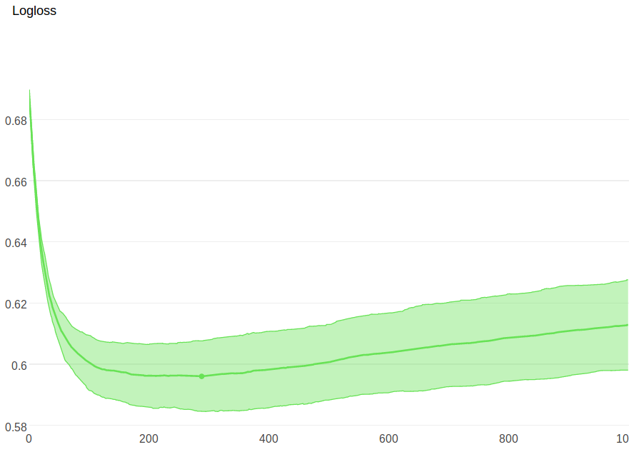
Training the model using catboost’s gradient boosting implementation yields optimal iterations of 288 with a logloss of 0.595 on out of sample data

Backtesting and Trading

Strategy 1:

As a first test, lets introduce a very simple strategy. define a confidence score for each match as:

C_team1 = (Model Imp Prob for Team1)/(Market Imp Prob for Team1)
C_team1 = (Model Imp Prob for Team2)/(Market Imp Prob for Team2)

If C_team1 > some_threshold, then place a bet on Team1, else if C_team2 > some_threshold, place bet on Team2. Else, do not bet.

Following the above rule for various threshold values and placing a constant bet of 50 GBP each time gives:

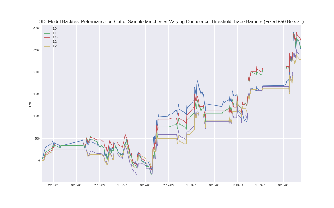
Note: In real life, for optimal bet-sizing in fixed probability settings like this, one should use the Kelly Criterion to determine betsize rather than a fixed amount.

As the confidence threshold increases, naturally, the volatility of the P&L path decreases since less bets are made. Clearly even this basic model vastly outperforms the market, albeit on the limited amount of ODI matches for which pricing is available.

UPDATE 2019-11-09: Strategy 2:

The above strategy is biased toward betting on low probability tail events and uses a flawed criteria. As an improved version, let p1 and p2 represent the market’s pricing for Team 1 and Team 2 respecitvely and let m1 and m2 be the model’s implied pricing for Team 1 and 2 (implied by the reciprocal of the class probabilities).

If:

Then choose Team 2

Conversely, if:

Then choose Team 1, for some pre-chosen epsilon In the case of neither of the above conditions being satisfied, then do not bet.

Using the above definitions, if Team 1 is chosen, the optimal Kelly betsizing as a fraction of current capital is given by:

And similarly for Team 2.

Below is a comparison of the P&L of Strategy 2 vs Random betting.

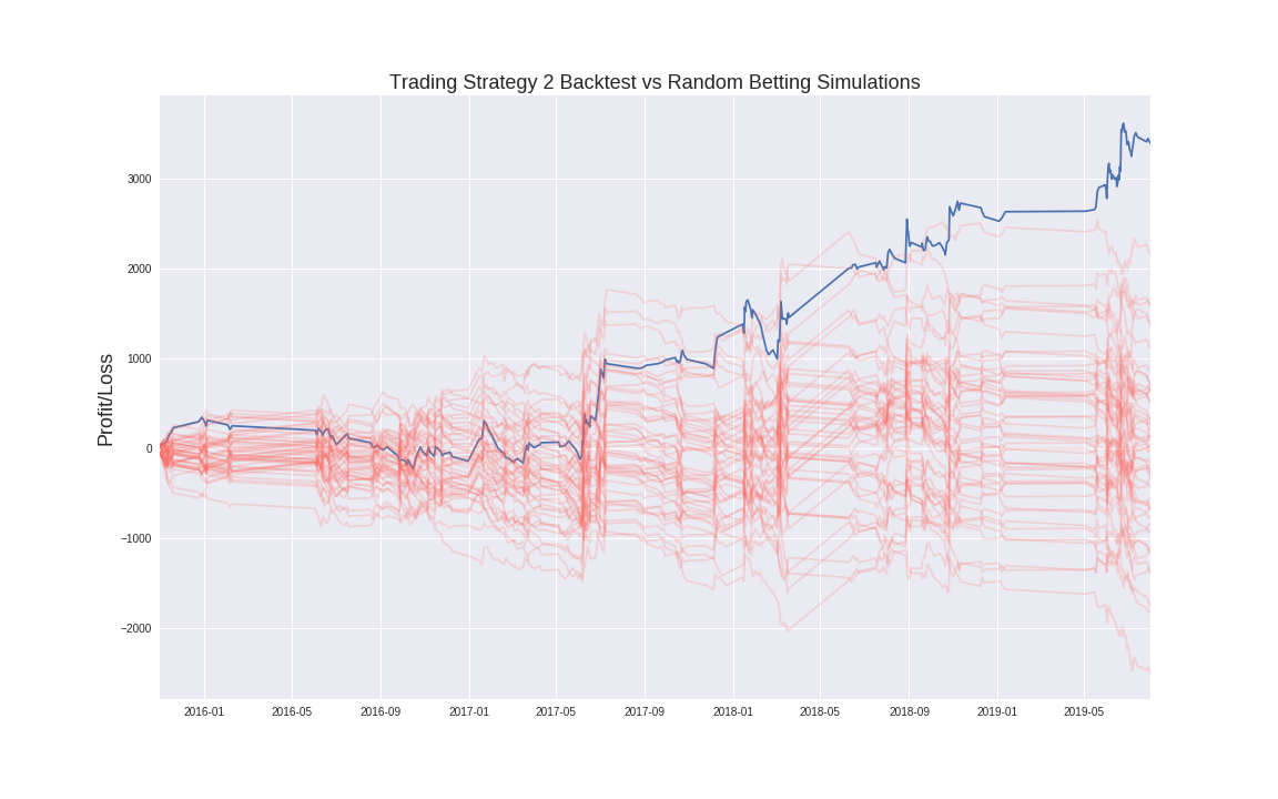
Achieving the results implied from this backtest is a 3.6 sigma event meaning that there is less than a 1% probability of achieving these results if following the baseline model (random betting).

A similar strategy can be used on other formats of cricket too, increasing the number of trading oppurtunities. This basic model does not perform any inplay trading, that is a topic for another day…

Other things not mentioned in this writeup required to make this basic strategy robust.

• Other formats of the game which add more pricing data
• Event driven inplay trading*
• Handling extenuating circumstance (key player injuries etc.)
• Automated bet placing
• In play stop losses
• Hedging
• Making markets when there is no liquidity using models prices.

Endnotes:

1: Betfair is an exchange rather than a bookie, meaning they provide a marketplace for individuals to set and take prices.

2: As an example, if Team1 is priced at 1.14 and Team2 is priced at 7.8, then this gives implied probabilities of (0.877, 0.128) for (Team1, Team2) respectively. Using these probabilities, betting at market odds would be defined as a simulation which would simply bet on Team1 87.7% of the time and Team2 12.8% of the time.

3: Admittedly, searching over k factor in this way is somewhat overfit, as hyperparameter tuning in this way is itself a form of overfitting – however, when using only subsets of the data, 26 seems like a very reasonable choice to maximising ELO’s prediction of match outcome.

4: Obviously we can only use the teams ELO from after the match played prior to the one in question