
Finding and Testing Parameters of the Vasicek Model.
The Vasicek Model is perhaps the simplest stochastic differential equation which is generally used to model short term interest rates or FX forward rates, however in theory it can be applied to any mean reverting asset such as commodities or FX spot.
\[dS_t = \lambda(\mu-S_t)dt+\sigma dW_t\]where \(S_t\) represents the asset price at time t and \(W_t\) is standard Brownian Motion.
The SDE takes three parameters:
\(\mu\) describes the mean level, which all trajectory paths should evolve around in long term behaviour.
\(\lambda\) is the speed of mean reversion
\(\sigma\) is the standard deviation, modelling volatility.
In this post, I look at EUR/USD mid-price data from 08/11/2015 to 01/12/2015 (excluding weekends) and force a solution via maximum liklehood estimation for the three parameters.
Continuous Solution
The continuous case solution to the Vasicek differential equation is obtained by observing:
\[d(e^{\lambda t} S_t) = e^{\lambda t}dS_t + \lambda e^{\lambda t}S_t dt\] \[= e^{\lambda t}[\lambda(\mu - S_t)]dt + \sigma e^{\lambda t} dW_t + \lambda e^{\lambda t}S_t dt\] \[\lambda e^{\lambda t} dt + \sigma e^{\lambda t} dW_t\]In integral form:
\[\Rightarrow e^{\lambda t} S_t = S_0 + \lambda\int^{t}_{0}e^{\lambda u}du + \sigma\int^{t}_{0}e^{\lambda u}dW_u\]Evaluating the deterministic integral yields:
\[e^{\lambda t} S_t = S_0 + (e^{\lambda t} -1) + \sigma\int^{t}_{0}e^{\lambda u}dW_u\]Dividing both sides by \(e^{\lambda t}\) and rewriting \(\lambda (s-t)\) as \(-\lambda (t-s)\) we get:
\[S_t = S_0 e^{-\lambda t} + (1-e^{-\lambda t}) + \sigma\int^{t}_{0}e^{-\lambda(t-s)}dW_s\]Discrete Time Analog
In this post, I am using 30 minute intervals over approximately 1 month, so we can simplify greatly. In discrete time, \(S_{t+1} = \alpha S_t + \beta + \Upsilon(\mu_1 , \sigma_1^2)\)
ie: a Linear dependence with an normally distributed random term.
To find the parameters, we observe the conditional probability distribution:
\[f(S_{t+1} | S_{t})\]This is distributed normally as: \(N(S_{t}e^{-\lambda}-\mu(1-e^{-\lambda}),\sigma^2 \frac{1-e^{-2\lambda}}{2\lambda})\)
Let \(\sigma_1^2 = \sigma^2 (\frac{1-e^{-2\lambda}}{2\lambda})\) for brevity.
This can be simulated in code and we can generate sample paths as shown:
def vasicek_path(mu, sigma, _lambda, starting, n_ticks):
# runs a simulated trajectory path with n ticks
# with given parameters and starting value
path = [starting]
for i in range(0,n_ticks-1):
s = np.random.normal(0, 1, 1)[0]
a = (path[i]*math.exp(-_lambda)) +
mu*(1-math.exp(-_lambda)) +
(sigma * math.sqrt( (1-math.exp(-2*_lambda)) /
(2*_lambda) ) ) *s
path.append(a)
return path
def plotter():
for n in range(4):
plt.plot(range(50), vasicek_path(1.,1.5,0.25,1,50),
alpha = 0.6, color = 'red')
plt.plot(range(50), vasicek_path(1.,1.,1,1,50),
alpha = 0.6, color = 'blue')
plt.title('Simulated Vasicek Trajectories')
plt.ylabel('S(i)')
plt.xlabel('i')
plt.show()
plotter()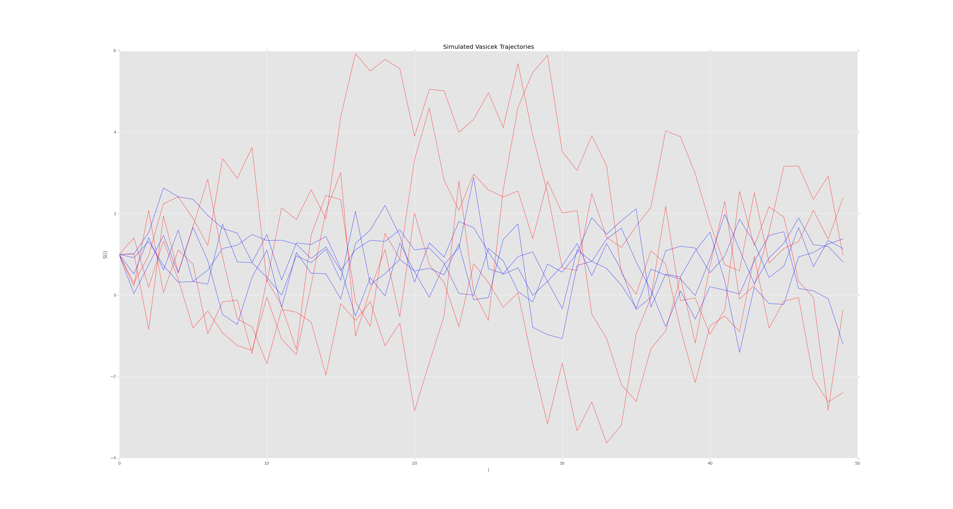 Red: \(\mu = 1, \lambda = 1.5, \sigma = 0.25\)
Blue: \(\mu = 1, \lambda = 1, \sigma = 1\)
The higher volatility of \(S_{red}\) is clearly visible with 50 sampling points.
Liklehood Estimation to find Parameters
The Liklehood Estimator is given by:
\[L(\mu,\lambda,\sigma_1) = \prod_{t=1}^{n} f(S_t|S_{t-1}) = \left( \frac{1}{\sqrt{2\pi\sigma^2}} \right)^n e^{-\sum^{n}_{t=1}(S_t - S_{t-1}\frac{e^{-\lambda} - \mu(1-e^-\lambda))^2}{2\sigma_1^2})}\]It suffices to maximise the Log-likehood estimator as the logarithm function is monotonically increasing and continuous.
\[log(L(\mu,\lambda,\sigma_1)) = \frac{-n}{2}log(2\pi\sigma^2) -\sum^{n}_{t=1} \frac{(S_t - S_{t-1}e^{-\lambda} - \mu(1-e^-\lambda))^2}{2\sigma_1^2} - n log(\sigma)\]Now, we partially differentiate \(log(L)\) with respect to \(\lambda\), \(\sigma_1\) and \(\mu\), setting the derivatives to zero gives us solutions for the estimator values.
For example, in the case of \(\mu\) we set:
\[\frac{dlog(L(\mu,\lambda,\sigma_1))}{d\mu} := 0\] \[\Rightarrow \mu_{est} = \frac{\sum^{n}_{t=1}(S_t-S_{t-1})e^{-\lambda}}{n(1-e^{-\lambda})}\]The case is similar for \(\lambda\) and \(\sigma_1\)
Plotting
Data was taken from Bloomberg Terminals at King’s College London
Plotting the Backtest Data (30 minute granularity, no weekend data)
dates = []
prices = []

with open('usdeur30min.csv', 'r') as csvfile:
    reader = csv.reader(csvfile)
    for row in reader:
        date_object = datetime.strptime((row[0]), '%d/%m/%Y %H:%M')
        dates.append( date_object )
        prices.append( float(row[1]) )

dates = dates[::-1]	  # Chronologically
prices = prices[::-1] #
Simulating Trajectories with Estimated Parameters
With the initial starting mid-price, 50 simulations are ran with the MLE parameters, along with the real data in red.
s_x = sum(prices[0:-1])
s_y = sum(prices[1:])
s_xx = sum(i**2 for i in prices[0:-1])
s_yy = sum(i**2 for i in prices[1:])
s_xy = sum(prices[i]*prices[i+1] for i in range(0,len(prices)-1))

mu  = (s_y*s_xx - s_x*s_xy)/( len(prices)*(s_xx - s_xy) - (s_x**2 - s_x*s_y) )

_lambda = -math.log( (s_xy - mu*s_x - mu*s_y + len(prices)*mu**2) /
					 (s_xx -2*mu*s_x + len(prices)*mu**2) )

a = math.exp(-_lambda)
sigmah2 = (s_yy - 2*a*s_xy + (a**2)*s_xx - 2*mu*(1-a)*(s_y - a*s_x) +
		  len(prices)*(mu**2)*(1-a)**2)/len(prices)
sigma = math.sqrt(sigmah2*2*_lambda/(1-a**2))

def forward_test():
    prices_path = [prices[0]]
    for i in range(0,len(dates)-1):
        s = np.random.normal(0, 1, 1)[0]
        a = (prices_path[i]*math.exp(-_lambda)) +mu*(1-math.exp(-_lambda)) +
        	(sigma * math.sqrt( (1-math.exp(-2*_lambda)) / (2*_lambda) ) ) *s
        prices_path.append(a)
    return prices_path

for n in range(1,30):
    plt.plot(dates, forward_test(),linewidth=0.4,alpha = 0.7, color = 'green')
plt.plot(dates, prices,linewidth=2.0, color = 'red')
plt.title('Mid Price of USD/EUR: 08/11/15 - 01/12/15')
plt.ylabel('USDEUR Mid Price')
plt.xlabel('Date')
plt.show()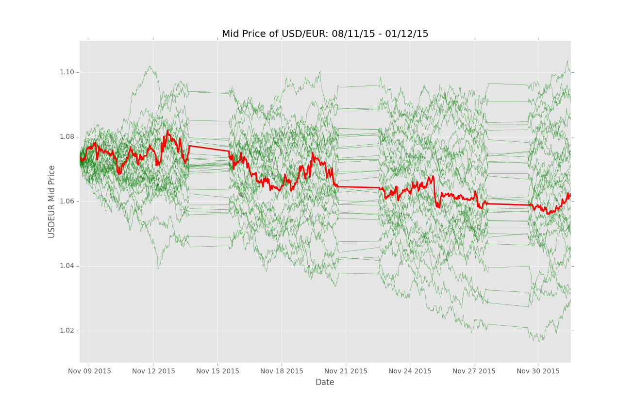
Note: the jumps are due to weekends.
Next Steps
The above results are not particularly surprising. Indeed we expect the final points of simulated trajectory paths to be normally distributed around the real data result. The next steps are to forward test our parameters with new unseen intra-day data. My next post will cover this in more detail once a month has elapsed.